
How to Plan a Geo-Experiment: KPIs, Duration, Geography and Budget
Planning a geo-experiment requires balancing statistical, budgetary, and business considerations. Statistically, the goal is to design a regional split that provides sufficient power given the available budget and test duration. In practice, however, the statistically optimal design may not be feasible because of budget constraints or business limitations on activating campaigns across regions. The key to effective planning is therefore finding the right balance among these considerations. This blog post walks through the key decisions involved in planning a geo-experiment and discusses how to weigh these trade-offs and validate that the final design provides a credible comparison between treatment and control.
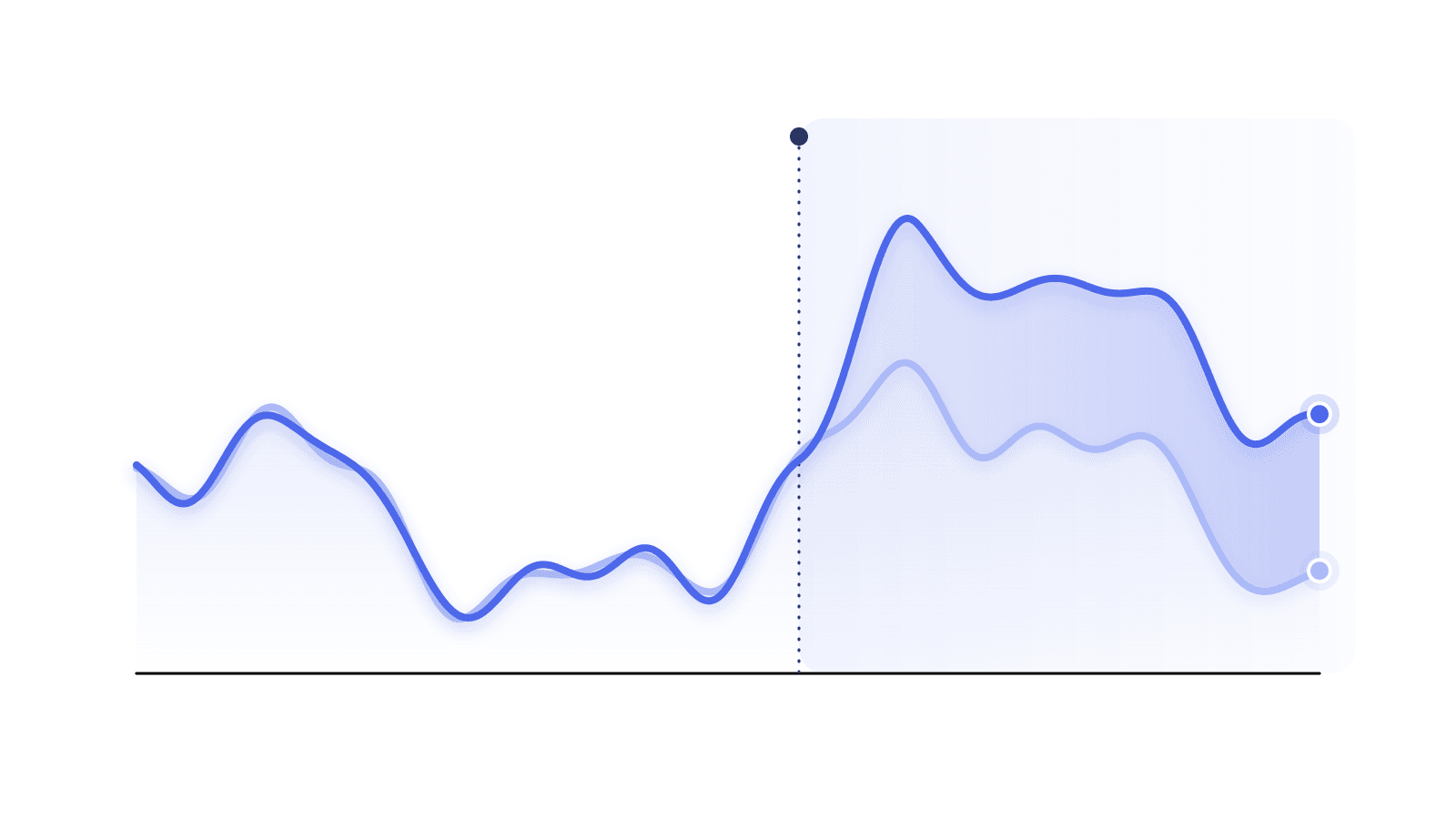
Planning a geo-experiment requires balancing statistical, budgetary, and business considerations. Statistically, the goal is to design a regional split that provides sufficient power given the available budget and test duration. In practice, however, the statistically optimal design may not be feasible because of budget constraints or business limitations on activating campaigns across regions.
The key to effective planning is therefore finding the right balance among these considerations. This blog post walks through the key decisions involved in planning a geo-experiment and discusses how to weigh these trade-offs and validate that the final design provides a credible comparison between treatment and control.

Figure 1. Geo-experiment design workflow. The experiment is designed based on a set of parameters that determine the test design, including how regions should be split between treatment and control and the required budget. If the resulting design is valid and within the available budget, the test can begin. Otherwise, the parameters are adjusted and the design process is repeated.
The Five Parameters Needed to Design the Experiment
#1: KPI Selection
Key performance indicators (KPIs) are the metrics that will guide the interpretation of the experiment results. In practice, strong experimental KPIs tend to share four key properties:
- Fast-moving: Respond quickly to exposure, enabling shorter experiments.
- Low noise: Have low variance across regions, making measurements more comparable.
- Stable variance: Show consistent variability over time.
- Business-relevant: Align directly with strategic outcomes.
KPI choice directly shapes the experiment’s power, duration, and feasibility. Action-based metrics such as conversions or installs are typically less variable, enabling smaller samples and shorter tests. Business outcomes such as revenue, spend, or profit are often more important but noisier, requiring larger samples and longer experiments to detect reliable effects.
#2: Test Duration
Test duration is closely related to time granularity, the period over which data are aggregated for each region. Analysts typically choose between daily and weekly aggregation. Daily data provide more observations and greater statistical power but are more sensitive to short-term noise. Weekly aggregation smooths these fluctuations but produces fewer observations and may require a longer test. Daily aggregation is generally preferred unless the data are too noisy for reliable inference.
The minimum recommended duration depends on the aggregation level: at least 14 days for daily data to capture complete weekly cycles and day-of-week effects, and at least four weeks for weekly data to provide sufficient observations for reliable inference.
Two additional factors may require a longer test window. First, allow for the ramp-up period required for the marketing algorithm or channel to reach stable performance, which may take one to two weeks. Second, account for conversion lag: if conversions occur days after exposure, extend the observation window beyond the end of the campaign to capture delayed effects. Ideally, the post-campaign observation period should be defined in advance.

Figure 2. Overall test window. Test duration should account for three periods: a ramp-up period for algorithm calibration, a core test period during which the campaign has reached stable performance, and a post-campaign observation period to capture effects that emerge with a delay.
#3: Geographic Granularity
In geo-experiments, the randomization units are geographic regions. Common choices include states or provinces (e.g., U.S. states, Canadian provinces, and German Bundesländer) and, in the U.S., Designated Market Areas (DMAs)—210 regions defined by shared media consumption patterns.
The choice of geographic granularity involves several trade-offs:
- Higher granularity (smaller regions) provides more units, increasing statistical power and enabling better synthetic-control matching, but may also increase measurement noise and spillover between neighboring regions.
- Lower granularity (larger regions) reduces noise and spillovers and improves treatment-control isolation, but provides fewer units for matching and may reduce statistical power.
Overall, DMAs or similar local-market definitions often offer a good balance between the number of units available for statistical power and counterfactual matching and the risk of noise and spillovers. However, the optimal granularity also depends on time granularity. With weekly aggregation, for example, there may be too few pre-test observations relative to the number of DMAs, making synthetic-control estimation less stable and computationally demanding. In such cases, coarser geographies, such as states, may be more practical.
#4: Treatment Share
Once geographic granularity is set, the next decision is how to allocate regions between treatment and control. By default, we recommend giving the optimization algorithm full flexibility to maximize statistical power while minimizing cost.
However, practical and business considerations may justify deviating from the statistically optimal allocation depending on the type of intervention. For an established marketing channel, companies may prefer to keep the channel active in most regions and use a small holdout group as a control. In contrast, when testing a budget increase or a new channel, a smaller treatment group may be preferable to limit financial exposure and operational risk.
#5: iCPA / iROAS Threshold
Designing a geo-experiment requires defining the minimum incremental impact needed to justify the additional spend. For action-based KPIs such as subscriptions, installs, or trials, this is expressed as iCPA (incremental cost per acquisition); for value-based KPIs such as revenue, as iROAS (incremental return on ad spend).
The algorithm uses the predefined cost-effectiveness threshold to calculate the minimum budget needed to determine whether the campaign's measured iCPA or iROAS meets the business requirement. This should be viewed as a minimum, not a target: a larger budget generally improves precision, enables detection of smaller effects, and produces narrower confidence intervals.
If the recommended budget exceeds practical constraints, consider three adjustments:
- Test duration: If daily spend is the constraint, extending the test spreads the required total budget over more days, lowering the daily spend needed.
- Treatment–control allocation: Adjusting the proportion of regions assigned to treatment can reduce the budget required to detect the desired effect.
- Temporal aggregation: If daily outcomes are noisy, weekly aggregation can reduce fluctuations and improve the signal-to-noise ratio, reducing the required budget. This is typically a last resort.
How Do I Know If My Design Is Good?
Treatment-control split
Once the test is designed, the final step is to validate that treatment and control regions provide a credible comparison. Using pre-test data, we examine the residuals, the KPI differences between treatment and control before the intervention. A well-designed split should produce residuals that are:
- Centered around zero, indicating no systematic bias between treatment and control regions.
- Stable over time, with no persistent upward or downward trends. Such drift indicates that the groups were already evolving differently before the intervention, making it difficult to attribute post-test differences to the campaign.
- Weakly autocorrelated, meaning that residuals behave approximately like random noise rather than showing strong dependence from one period to the next. High autocorrelation suggests that important patterns remain unexplained, which can compromise inference.
When these conditions are met, treatment and control regions exhibit similar pre-test behavior, increasing confidence that differences observed during the test can be attributed to the campaign.

Figure 3. Pre-test residual diagnostics. Pre-test residuals, defined as the difference between treatment and control outcomes, under a well-balanced design (desired pattern of residuals, top left) and when the residuals violate the requirements for a valid allocation (not centered around zero, top right; drift, bottom left; autocorrelation, bottom right).
Beyond examining the residuals, the design can be evaluated by mimicking a “test” period during the study-design stage. To do this, the training data are split into two parts (e.g., 80% and 20%). The larger portion is used to train the model and select the experimental design. The remaining data are then used for validation: regions are assigned to the treatment and control groups according to the selected design, and the difference between the groups is evaluated as if this were the actual test period.
Importantly, unlike in the actual test period, where we expect to detect an effect of the campaign, the validation period should show no systematic difference between the groups. A meaningful difference would suggest that the selected design does not adequately balance the regions and may produce biased estimates of the campaign effect.
Budget
Beyond the regional split between treatment and control, the second key output of the design process is the required test budget. This budget is determined through statistical and mathematical calculations, but it should also be validated against business considerations before the test begins. Two complementary considerations are particularly important. First, the required budget must be feasible given the available budget. Second, it should be representative of the level of marketing activity the business would normally undertake. Although shorter tests are generally desirable, shortening the test duration may require substantially higher daily spend to achieve sufficient statistical power. A test may therefore be statistically well designed but impractical if the required budget is too high or does not reflect realistic marketing activity.
Take-home message
In this blog, we provided a practical guide to the main decisions involved in planning a geo-test and how to navigate the trade-offs between methodological best practice and operational constraints. This serves as a starting point for those looking to transition from traditional experimentation to geo-experiments, and as a foundation for leveraging this powerful tool for causal inference in real-world settings.
Geo Testing at Bell Statistics
We plan, run and analyse geo experiments to measure what your marketing actually caused.
See how we work on geo testing →More on geo testing
All posts →
Six Tips for Running Geo Experiments the Right Way
It is often said that experience is the best teacher, and geo-testing is no exception. Running high-quality geo-experiments involves a learning curve, where performance improves with practice and accumulated knowledge. In this blog, we crystallize our experience from conducting dozens of geo-tests across the industry into six practical tips. This is essential reading for anyone who not only wants to run geo-experiments, but to run them the right way.


GeoLift vs. Meridian GeoX vs. Bell: Three Approaches to Geo Experimentation
Designing a high-power geo experiment is difficult, and there is no single methodology that is best in every setting. Here, we compare GeoLift, Meridian GeoX, and Bell to see how their different approaches to design, counterfactual estimation, and inference play out in practice.


Geo Experimentation: How to Measure the Incremental Impact of Marketing
Marketing is a high-risk, high-reward investment for companies. On the one hand, effective marketing can have a significant impact on a product’s growth. On the other hand, marketing often involves massive budgets, making it critical to invest those resources where they can generate the greatest impact. As analysts, our goal is to determine whether, and to what extent, marketing investments actually drive incremental impact. How can we do that? In this blog, we introduce geo experiments, a powerful statistical approach for measuring the incremental impact of marketing campaigns. We’ll walk through what geo testing is, when it should be used, and why it can provide a more reliable measure of causal impact than common attribution models. If you’re looking for a robust way to measure the true impact of your marketing campaigns, this is where you should start.