Network effects exist when a product becomes more valuable as more people use it. They make an experiment systematically understate a change's launch impact, because a variant tested on a fraction of users never reaches the scale that produces the benefit.
Also called
network externalities, demand-side economies of scale, viral effects
A network effect exists when each additional user makes the product more valuable to everyone else. A messaging app is useless to one person and indispensable to a company where everyone is on it; a marketplace with more sellers attracts more buyers, which attracts more sellers. The property is about the product rather than about measurement — but it creates a measurement problem that no amount of statistical care resolves.
The problem is that an experiment tests a variant at partial adoption and the launch happens at full adoption. If a feature's value depends on how many of your contacts also have it, then a 50% test measures the feature at 50% penetration, and the launch delivers it at 100%. Those are different products. The experiment is not biased in the usual sense — it correctly estimates the effect at the tested scale — it just estimates a quantity that is not the one the decision needs.
The direction is almost always understatement for genuinely network-dependent features, and the size of the gap depends on how steeply value rises with adoption. A collaboration feature that requires both parties is worth roughly nothing when only half of each pair has it, so a user-randomised test can measure close to zero on something transformative. This is one of the few situations where a null experimental result is genuinely weak evidence of no effect.
It is worth separating this from interference, which the two are frequently conflated with. Network effects are the product property: value grows with adoption. Interference is what that property does to the arithmetic of your experiment by carrying treatment across the boundary between arms. One is a business phenomenon, the other is the measurement failure it causes — and keeping them distinct makes it clearer that the response is a design change rather than a different feature.
The designs that recover the real quantity all work by making the treated region large enough to contain the network. Cluster randomization by workspace or friendship group gives full adoption inside each treated cluster. Geographic randomisation does the same at market scale. Both cost heavily in power, and a staged rollout with careful before-and-after measurement is sometimes the only feasible option — with all the weaknesses that implies for the counterfactual.
The formula
The dependence on adoption is what distinguishes this from an ordinary effect, and it is why the tested quantity and the launch quantity differ.
Value depends on adoption
V( user ) = f( n adopters ), f increasing
The defining property. For an ordinary feature f is flat and the problem does not arise.
What the experiment measures
effect at treatment share p, not at p = 1
A 50/50 test measures the feature at 50% penetration. The launch is a different condition.
The pairwise case
P( both parties treated ) = p²
At p = 0.5 only a quarter of pairs are fully treated, so a two-sided feature measures near zero.
A messaging product tests a feature that only works when both people in a conversation have it. It is run first as a 50/50 user-level test, then as a cluster-randomised test over 2,400 organisations.
User-level test: measured effect
+0.4% on messages sent, p = 0.41
Conversations with both parties treated
25% (0.5²)
Conversations with exactly one treated
50% — feature unusable
Cluster-randomised: measured effect
+6.8% on messages sent
Cluster-randomised interval
+2.1% to +11.5%
Clusters required for that precision
2,400 organisations
The user-level test found nothing at p = 0.41. The clustered design found a 6.8% lift on the same feature.
The second and third rows explain the first entirely. At a 50/50 split only a quarter of conversations had the feature on both sides, and in half of them one party had something the other could not use — which is arguably worse than not shipping it. The user-level test correctly measured the feature at 50% penetration, and that quantity is close to zero because the feature does not work at 50% penetration. It is not a false negative in the usual sense; it is an accurate answer to a question nobody wanted asked. The clustered design gives every user in a treated organisation the feature, so treated clusters experience it as they would after launch, and the 6.8% is the number that predicts the rollout. The cost is visible in the interval — 2,400 clusters is far less information than 40,000 users — and it is worth paying because the alternative was a precise zero.
Common misconceptions
דA null result means the feature does not work.”
For a network-dependent feature it may mean the test could not represent the launch condition. A feature requiring both parties is worth little at 50% adoption, so a user-randomised test measures close to nothing regardless of how valuable it becomes at full rollout. This is one of the few cases where a null experimental result is genuinely weak evidence.
דNetwork effects and interference are the same thing.”
Network effects are a property of the product — value rising with adoption. Interference is what that property does to an experiment by carrying treatment across the arm boundary. Keeping them separate clarifies that the response is a change of design rather than a change of feature.
דYou can extrapolate from a 50% test to a 100% launch.”
Only with a model of how value scales with adoption, which you rarely have and which is the hard part of the problem. The relationship is usually non-linear and sometimes has a threshold below which the feature is worthless. Extrapolating linearly from a partial-adoption measurement is guessing with extra steps.
Frequently asked questions
Which experiment design handles network effects?
One where the randomisation unit contains the network. Cluster by organisation, team or friendship group so treated clusters reach full adoption internally; randomise by geography where the network is regional. Both cost substantial power because the effective sample becomes the number of clusters. Where even that is infeasible, a staged rollout with careful before-and-after measurement is the fallback, with all the counterfactual weaknesses that carries.
How do I tell a genuine null from a network-effects null?
Ask whether the feature's value depends on other people having it. If it requires two parties, a 50/50 test leaves only a quarter of pairs fully treated and the measured effect will be near zero whatever the feature is worth. Checking the effect among users whose contacts happened to be treated is a useful diagnostic — not a valid analysis, since that group is not random, but it usually settles which situation you are in.
How do network effects show up in a marketplace?
Two ways, pulling in opposite directions. Genuine network effects mean more sellers make the platform better for buyers, so a partial test understates a full launch. Competition for fixed supply means treated buyers take inventory from control buyers, so a partial test overstates it. Marketplaces frequently have both at once, which is why switchback and geographic designs are standard there rather than optional.
Applying it to a live measurement problem is the part that goes wrong. If you are designing an experiment, reading a result you do not trust, or trying to work out what your marketing actually caused, that is the work we do.
References
Katz, M. L., & Shapiro, C. (1985). Network Externalities, Competition, and Compatibility. American Economic Review, 75(3), 424-440.